Optimal Quadratization
Bychkov and Pogudin’s paper Optimal monomial quadratization for ODE systems recently showed up in my life to solve a problem my friend and I had been working on for a while, and whose name (quadratization) we did not even know! It goes something like this (and all examples here are taken from their paper):
You have a system \(\bf{x}\) of ODEs, with variables \(x_1, x_2, ..., x_n\) that are all polynomial, autonomous, and first order. Let’s say the degree of a monomial is the sum of the degrees of variables in the monomial, e.g. \(deg(x^3y^2) = 5\). The right hand side, though polynomial, has no restriction on the degree of any of the monomials appearing there. So, you might see something like this :\(x_7' = ... + x_8^2x_9^{12}x_{13} +...\) It’s a finite system, so it will of course have one or more maximal polynomials, thus there is a highest degree among them. Note, and this might matter later, that there might be different monomials that are ‘incomparable’ and share the highest degree:
If \(\bf{x}\) is a set of ODEs expressed as right hand sides that are sums of monomials $m$ then the set of incomparable terms (or peaks) of the system is the antichain
\(peak(\bf{x})=\) \(\{m \mid \text{m in }\bf{x}\) and \(\forall m' \neq m\) in \(\bf{x},\) \(m \not\leq m'\) and \(m' \not\leq m\}\).
and that might have more than one monomial in it.
The goal
The goal (our application) is to transform \(\bf{x}\) into a system of maximum degree equal to 2. So, how?
The big trick (or family of tricks) is: substitute variables! If I make a new variable, for example \(y_1 = x_8^2x_9^{12}x_{13}\) then I can freely rewrite the equation above as \(x_7' = ... + y_1 + ...\) and problem solved? Of course not! Because the variable \(y_1\), having been added to my system, must be defined in the ODE system, and it itself has to be quadratic. If we were to write out its own ODE, we’d get \(y_1' = 2x_8 \cdot x_8' \cdot x_9^{12} x_13 + ....\) following the chain rule. In a sense this is even worse than the original situation we were in (\(x_8'\) is going to contribute some potentially very high degree to this new ODE!)!
For now, note that
- In the example above, we did not even split the monomial up. We just renamed it.
- We can play this trick in many different ways, some more clever than others and our options depend on how much degree we allow terms to have in the final system. The specific problem here is quadratization, but if we were ok with having degree-3 monomials, we could look at ways to split them up three ways. Even with two degrees’ worth of ‘room to dance’, we have a lot of choices we can make about how we split up that monomial, let’s call it \(m = y_1 = x_8^2x_9^{12}x_{13}\).
For example, we could also have split it up into these two terms: \(m = x_8 x_9^6 \cdot x_8 x_9^6 x_{13} = y1 \cdot y2\) and note that in this case we have two ‘components’ that each have about half the degree of the original term. That is a more promising method, and when we go on to define their ODEs \(y_1 ' = (x_8x_9^6)'\) and \(y_2' = (x_8x_9^6 x_{13})'\) and after we spell these out using the chain rule, we’d see that the degrees of monomials in these polynomials are tending downward as we repeat the process.
The authors express this as follows:
If the system in question is \(\bf{x} = f_1(\bf{x}), f_2(\bf{x}), ..., f_n(\bf{x})\) then let \(D_i\) be the largest degree of the individual variable \(x_i\) over all of the \(f_i\). Then take the set \(M\) of all conceivable monomials \(x_1^{d_1} x_2^{d_2}....x_n^{d_n}\) where the \(0 \leq d_i \leq D_i\).
The ‘right choices’, which result in the fewest total new variables introduced into the system, for decomposing the system into degree 2 polynomials are somewhere in this set $M$ - the whole set of selections of monomials that account for both the original monomials and for new ones. This is the optimal decomposition or in the case of quadratizations, the optimal quadratization.
But the catch is surprising! \(M\) does not in general contain the optimal set of monomial choices for decomposing the original system quadratically. The thing is, one may benefit from jumping outside of \(M\), or in other words - choosing larger exponents than \(D_i\) for some variable \(x_i\).
Here’s one way to put it:
The (bounded) lattice at peak \(\bf{a} = [i_1,i_2,...,i_n]\) is the partially ordered \((\leq)\) set \(L(\bf{a})\) of all vectors \(\bf{b} \in \mathbb{N}^n\) satisfying \(\bf{b} \leq \bf{a}\).
So another way to ‘see’ it is that \(M\) defines a lattice, more specifically some overlapping lattices each terminating at the elements of \(peaks(\bf{x})\), but that lattice lives inside the simplex \(\Delta = \{ \bf{v} \in \mathbb{N}^n : \sum_i \bf{v}[i] \leq k \}\), where \(k\) is the highest degree among monomials in the system. I’m just naming it \(\Delta\) because its faces are triangles if there are only 3 variables. To see what I mean, look at some of these pictures. \(\Delta\) is blue, peaks are red, lattices are orange.
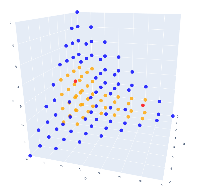
And here, purple are the partials resulting from the chain rule (without the associated derivatives multiplied onto them).
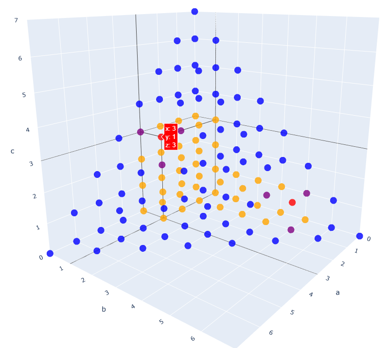
Peaks don’t have to live on any of the faces of \(\Delta\). For example, \([1,2,1]\) would be a peak, as it’s clearly \(\leq\)-incomparable to \([3,1,3]\). - but it’s not on any face.
An example from the paper
Lets look at Example 3 from Bychkov & Pogudin 2025:
Consider the system
\[x_1' = x_2^4, \qquad x_2' = x_1^2.\]The unique optimal monomial quadratization is the introduction of the following variables
\[z_1 = x_1 x_2^2, \qquad z_2 = x_2^3, \qquad z_3 = x_1^3,\]and the rewriting of the original system in their terms, giving the quadratic system
\[x_1' = x_2 z_2,\] \[z_1' = x_2^6 + 2x_1^3 x_2 = z_2^2 + 2x_2 z_3,\] \[x_2' = x_1^2,\] \[z_2' = 3x_1^2 x_2^2 = 3x_1 z_1,\] \[z_3' = 3x_1^2 x_2^4 = 3z_1^2.\]Since \(z_3 = x_1^3\) has \(x_1\)-degree \(3\), exceeding \(D_1 = 2\), this quadratization is not contained in
\(M := \{x_1^{d_1}x_2^{d_2} \mid 0 \le d_1 \le D_1,\ 0 \le d_2 \le D_2\},\) so it cannot be found by a search restricted to \(M\).
However, it does live in the associated simplex because the highest degree among all monomials in the original system is 4, and in the resulting system the highest degree is the same, and among new variables only 3.
The authors mention that for their examples, the set \(\hat{M} = \{x_1^{d_1}...x_n^{d_n} : 0 \leq d_1,....,d_n \leq D\},\) where \(D = \max_i D_i\) was sufficient. I’d be surprised if this is the case in general, I think! Note that \(\hat{M} \subset \Delta\) .
I’m not sure I see it - but I’m also kind of slow to pick up on things. So that’s not a claim about anything but me, at this moment of typing.
A natural question is: is there any benefit to going outside of \(\hat{M}\) ever? (or hell, why not leave the simplex too? go wild) If we have a monomial in the original system of degree, say, 17 - is there any utility in introducing a term of degree, say, 18? Or perhaps for a monomial like \(x^{15}\) is it worth going up to the nearest power of 2 above, allowing one to repeatedly halve powers ‘downward’? Can you find \(\epsilon\)-good decompositions doing this that aren’t optimal, even if the optimal ones - which might be hard to find in general - always live inside \(\hat{M}\) (yet to be established for sure)?
Anyway
Their approach goes something like this:
-
Follow a branch and bound strategy exploring the space of all possible quadratizations, with the objective function seeking the fewest number of new variables to be introduced.
-
Each subproblem consists of the the variable set \(V\) containing \(1, x_1, ..., x_n, z_1, ..., z_l\) where \(z_i\) are the new variables, and the set \(NS\) which contains all monomials appearing in any derivative of any variable in \(V\) which can’t be expressed as a product of two elements of \(V\). For example, if \(z_1 = x^3\) then \(z_1' = 3x^2 x' = 3x^6 + 5x^5\) and since \(x^5\) cannot be expressed as any two-element product of \(\{1,x,x^3\}\), it goes to variable jail. If \(NS\) is empty, then \(V\) is a quadratization.
-
Subproblems are constructed based on NS by picking an element \(m = x_1^{d_1}....x_n^{d_n}\) from \(NS\) that minimizes \(\prod_i^n (d_i + 1)\) . This “incentivizes” choosing a monomial where some of the individual degrees are minimal and others are larger. Note that (looking at monomials as tuples again,) (2,3,2) is a worse choice than (1,4,2). Whatever monomial is chosen, look at every decomposition of that monomial into \(m = m_1m_2\). Define a new subproblem for each such decomposition by adding \(\{m_1,m_2\}\setminus V\) to the variable set.
the rest of the paper describes pruning rules for the algorithm. To me, the most interesting thing is the above minimization function! I always though we’d be better off cutting monomials “in half” across all variables. I was wrong! And the reasons are themselves very interesting - the kinds of monomial decompositions that minimize that product determine the order in which subproblems are investigated by the algorithm and allow the authors to argue that any optimal subproblem of \(z_1,...,z_n\) is a solution of at least one of the children subproblems chosen by minimizing the product.